Getting rid of duplicate protein sequences becomes important when you are trying to annotate metagenomes. Redundant sequences can compete for reads when mapping to onto genes and don’t add anything extra information when assessing the functional capacity of a group of organisms. Probably the best way to remove identical or highly similar sequences from a FASTA file is through clustering homologous genes. I’ll show some results on data reduction from clustering experiments I ran on a single gene from many organisms and give you my opinion on when, and when not, to be stringent be be when clustering.

The platform I use to do my peptide sequence clustering is CD-HIT. It’s blazing fast and extremely simple to use. Basically, their algorithm clusters sequences based on word count overlap. What this means is that the user specifies a word size, meaning how many consecutive amino acids to consider at a time, and a percent identity as a cutoff on how similar sequences need to be to cluster together. CD-HIT starts by ordering the sequences from longest to shortest, then splitting each sequences into all posible words of the given size. It then counts the number of times each word appears in each sequences, giving each peptide a “signature” of abundances. The benefit of this step is twofold. First, it greatly simplifies each sequence to a small array, reducing the amount of memory needed to process each sequence. It also provides a very simple metric of comparison between peptides. The more their word counts overlap, the more similar they are. This idea was studied more in a study from back in 1998. If sequences fall within the user provided identity, then they are clustered together. Otherwise, a new cluster is formed. This happens processively until all peptides are put either into an existing cluster or make new ones. This procedure is known as greedy incremental clustering.

It’s easy to run CD-HIT once it’s installed. Here’s the command I used:

cd-hit -i metagenome.genes.peptide.fasta  -o metagenome.genes.peptide.99 -c 0.99 -n 5 -M 44000 -T 8

Here’s what each of the arguments mean:

1
2
3
4
5
6
-i = input FASTA file
-o = output file names
-c = percent identity (99%)
-n = word length
-M = allowed memory usage in Mb (=44 Gb)
-T = number of threads for parallelization

CD-HIT produces 2 files as output: a FASTA file of the first member added to each cluster, and a text file listing which sequences from the original FASTA belong to each cluster.

For a test case, I looked to a paper from synthetic biology. A group used data from systematic deletion experiments to define the minimal list of genes to function as a free-living bacterial genome. What resulted was a list of genes that have some homolog in many, if not all, bacteria. Using one of these genes makes for a great way to test how how many sequences are clustered together as the minimum percent identity is decreased. I chose adenylate kinase (adk), and downloaded the protein sequence for 200 bacterial homologs to a FASTA file from NCBI.

I performed a range of percent identity clusterings from 100% to 70% using the same word size of 5. Below is a summary of the results:

1
2
3
4
5
6
7
8
9
10
11
12
13
14
15
16
17
18
19
20
21
22
23
24
# Original FASTA
# Total sequences:  200
# Fraction of original: 100%

# Following clustering:
# Percent identity:  100%
# Total sequences:  186
# Fraction of original:  93.0%

# Percent identity:  99%
# Total sequences:  183
# Fraction of original:  91.5%

# Percent identity:  90%
# Total sequences:  178
# Fraction of original: 89.0%

# Percent identity:  80%
# Total sequences:  156
# Fraction of original:  78.0%

# Percent identity:  70%
# Total sequences:  130
# Fraction of original:  65.0%

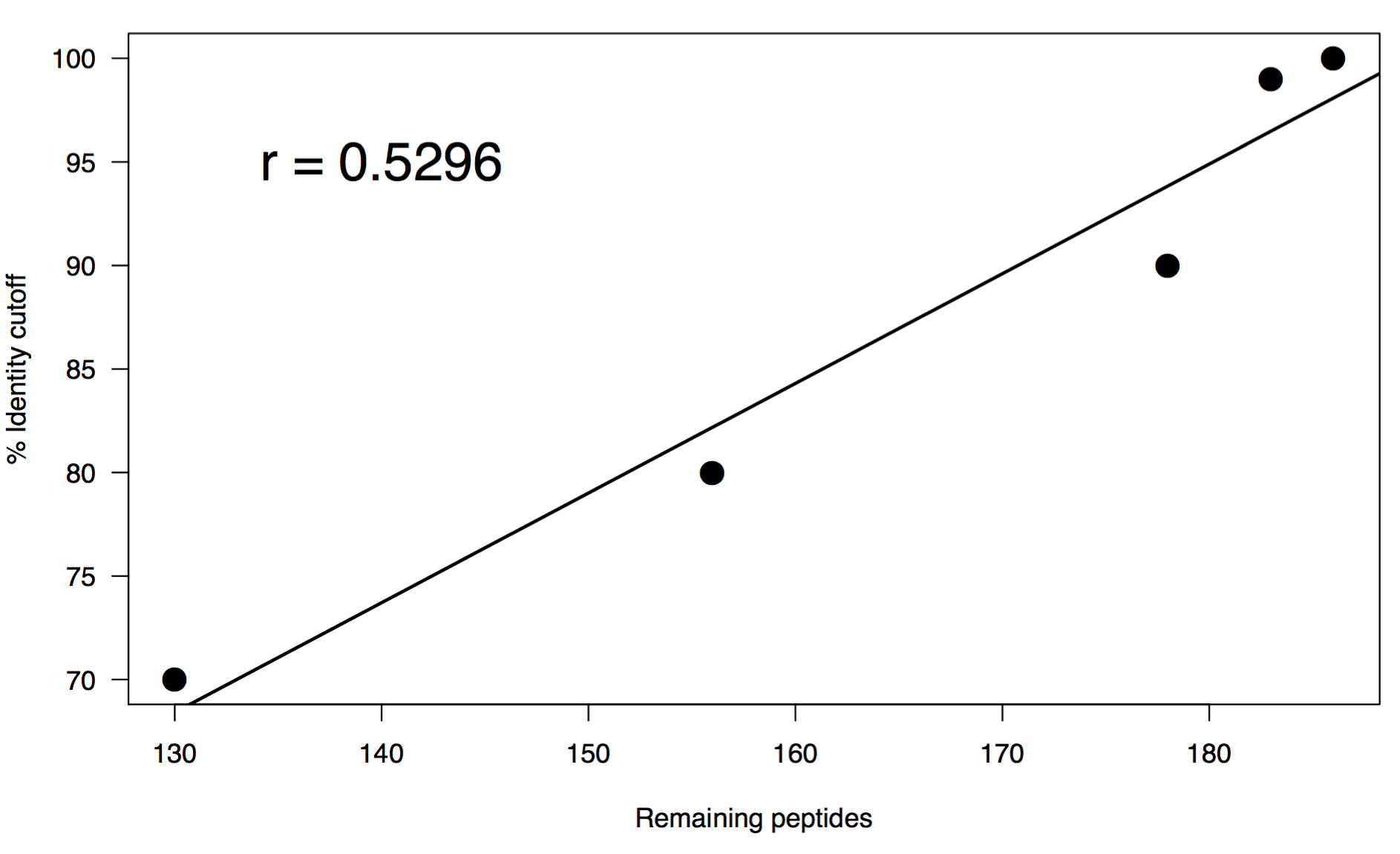
These results are interesting in that there is a pretty swift drop off even clustering at 100%. This may not be all that surprising since they do all come from the exact same gene, but you could also expect a greater level of diversity on adk across species. You may be able to chalk this up to how well the gene is conserved so it’s sequence might only deviate slightly. After this initial droff, there is a linear relationship in the rate at which sequences cluster vs percent identity cutoff. I think that what it comes down to in the end is if you are trying to capture the full repetoire of sequence diversity of homologs in a metagenome, or if you want to look at the relative functional capacity of a collection of genes. Either way, some amount of dereplication is necessary to avoid genes equally competing for reads when you reach the mapping steps of your analyses.

I was recently talking with Geof Hannigan, a postdoc in our lab, and he pointed out a pretty critical piece of information I had been overlooking. When sequencing reads become long enough, you may sequence passed the fragment size and into the 3’ adapter. This is especially problematic when you move on to assembly because these introduced sequences will have 100% homology to one another and assemble on the adapter instead of actual genome sequence. Similar problems can arise in a couple different ways as shown in the figure below. These artifacts will leave you with contigs that don’t reflect biology at all.

To avoid this I am now using a program called Cutadapt, where the figure came from, to remove any residual adapter sequences from my reads prior to assembly. The program requires python 2.7 and the command to run it looks like this:

1
python2.7 /mnt/EXT/Schloss-data/bin/cutadapt-1.9.1/bin/cutadapt --error-rate=0.1 --overlap=10 -a CAAGCAGAAGACGGCATACGAGATTAAGGCGAGTCTCGTGGGCTCGG -A GACGCTGCCGACGAGCGATCTAGTGTAGATCTCGGTGGTCGCCGTATCATT -o read_1.trimmed.fastq -p read_2.trimmed.fastq read_1.fastq read_2.fastq

Each argument supplies the following info:

1
2
3
4
5
6
7
8
--error-rate = Rate for how generously you still call a matching sequence, basically 1 in 10 bases can be a mismatch
--overlap = Minimum number of overlapping bases to call a match
-a = 5' sequencing primer full sequence, adapter + index
-A = reverse complement of the 3' sequencing primer 
-o = Output file name for read 1 followinf trimming
-p = Output file name for read 2

The last two file names without options before them are the forward and reverse read files

In order to get the reverse complement of the 3’ adapter, I wrote a small python script to reverse the order of a nucleotide sequence and then switch each base to it’s complement. Below is what it looks like and I’ve hosted on the Github page I made for scripts I talk about on my blog. This new adapter trimming step is critical for both my metagenomic and metatranscriptomic pipelines, basically anything with some amount of random fragment size. Otherwise the primer fragments left in the data negatively impact and assembly or mapping you try to do downstream.

#!/usr/bin/env python

# Computes the reverse complement of a given nucleotide string
# USAGE: rev_comp.py input_sequence


import sys

def reverse_complement(nucleotides):

	seq_str = str(nucleotides).upper()
	rev_seq_str = seq_str[::-1]

	pyr_seq_str = rev_seq_str.replace('A', 'n')
	pyr_seq_str = pyr_seq_str.replace('T', 'A')
	pyr_seq_str = pyr_seq_str.replace('n', 'T')

	final_seq_str = pyr_seq_str.replace('C', 'n')
	final_seq_str = final_seq_str.replace('G', 'C')
	final_seq_str = final_seq_str.replace('n', 'G')

	return final_seq_str


print(reverse_complement(sys.argv[1]))

Below are some stats from the assembly of the same 250 bp paired-end dataset from a HiSeq, just with and without the trimming protocol I laid out above.

Without 3’-adapter trimming:

1
2
3
4
5
6
7
8
9
10
11
Total sequences: 431204
Total bases: 495.00 Mb
Sequence N50: 1762
Sequence L50: 28
Sequence N90: 452
Median sequence length: 560
Interquartile range: 436
Shortest sequence length: 250
Longest sequence length: 420252
Sequences > 1 kb: 88470
Sequences > 5 kb: 10866

With adapter trimming:

1
2
3
4
5
6
7
8
9
10
11
Total sequences: 496917
Total bases: 471.39 Mb
Sequence N50: 1434
Sequence L50: 44
Sequence N90: 369
Median sequence length: 474
Interquartile range: 423
Shortest sequence length: 250
Longest sequence length: 201752
Sequences > 1 kb: 83535
Sequences > 5 kb: 10603

The assembly quality doesn’t seem to have changed dramatically, however the best metric is really how many reads map to the contigs that you just assembled. Prior to this trimming <49% of reads mapped at least once to a contig. Now >70% are mapping! That’s a huge improvement! The new contigs should reflect what I actually sequenced and allow for a better analysis from now on.