I’ve been pretty excited to talk about another angle I’m working for my project, and that is to try and
look at the nutrient niche of bacteria in the gut by using metabolic models built from an organism’s genomic
information. Inferring aspects of an organism’s ecology and how it may impact other species in its environment
based on high-throughput sequence data has been called Reverse Ecology.
I started this project after reading a pretty cool review from Roie Levy and Elhanan Borenstein.
Their lab used an approach where they used a decomposition algorithm on metabolic networks to identify substrates or nutrients
that a bacteria needs to obtain from its environment. They went on to use this information to accurately predict community
assembly rules in mouth-associated bacterial communities. I used their methods
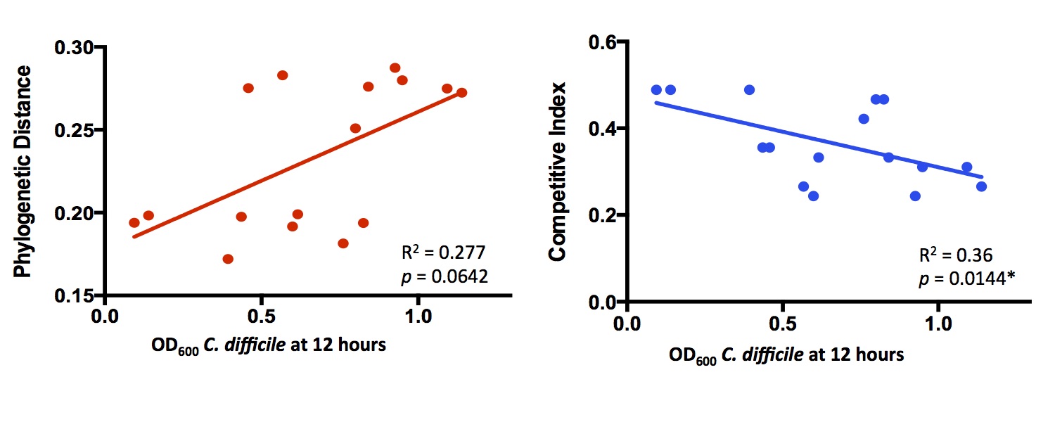
and found that comparing substrate lists between species predicted in vitro competition more accurately than phylogenetic
distance. Here’s a little bit of the data:
Each point is a separate bacterial species, competed against C. difficile in rich media. Competitive Index refers to
how much overlap there is between metabolic networks. I didn’t follow this up much further to focus on other projects,
but we may come back to it in the future.
What I’ve been working on more recently has been integrating transcriptomic data into genome-scale metabolic models. The
methods I’m using are loosely based on some work I read out of Jen Nielsen’s lab.
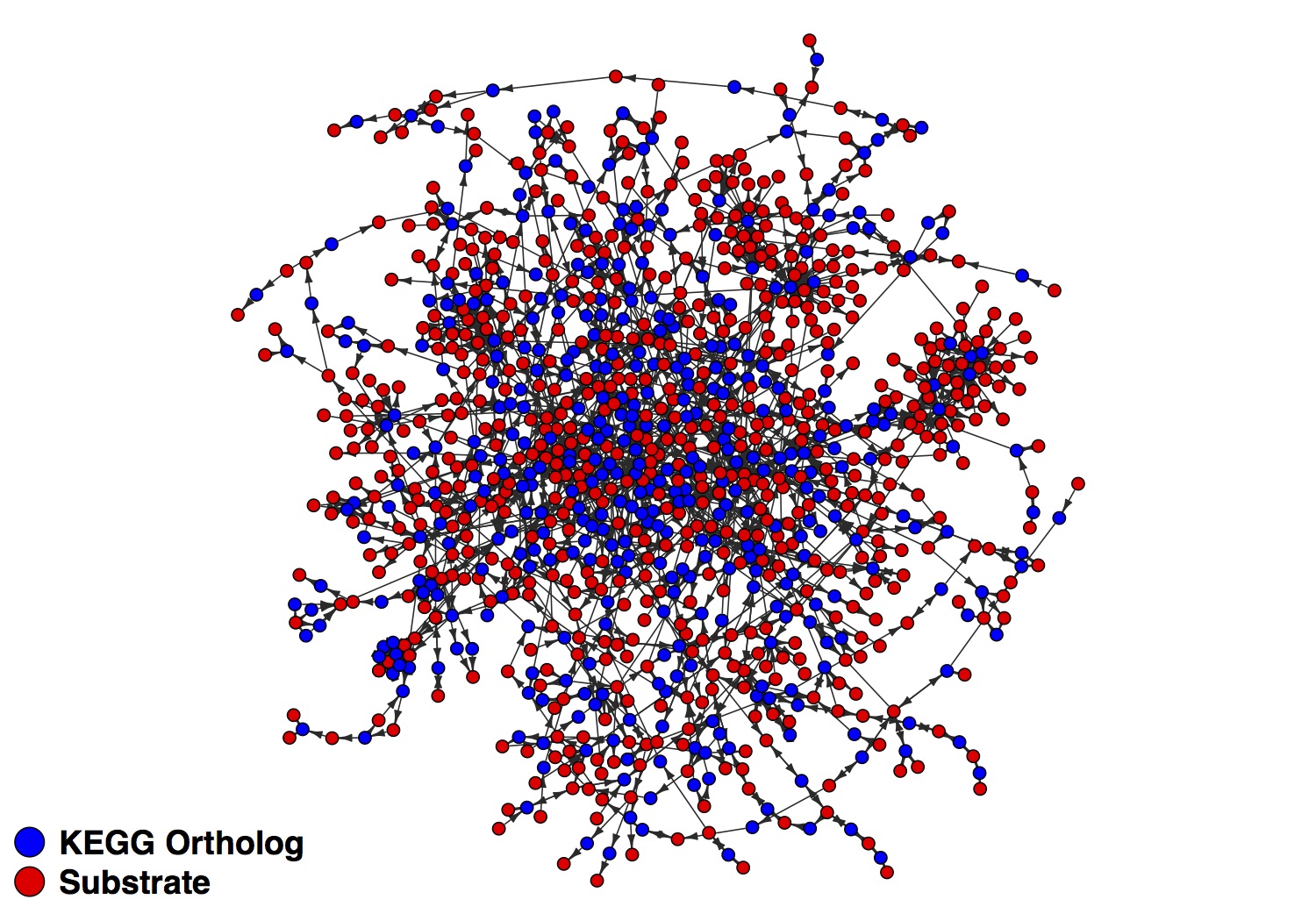
Their approach used a bipartite network architecture with enzyme nodes connecting to substrate nodes. Since substrates only
directly connect to enzyme nodes, you are then able to map transcript abundance to their respective enzymes and then make
inferences about how in-demand the substrates they act on are. Here’s part of one network I’ve generated as an example:
After mapping transcripts to the enzyme (KEGG ortholog) nodes, you can get a read on how important the adjacent substrate nodes are. I’m
extending this to infer the nutrient niche of species in the gut. We are working on the analysis and manuscript now so I’ll
have a lot more to post soon.
For now, here’s the R code I used to generate the network plot:
# Load igraph packageinstall.packages("igraph")library(igraph)# Define variablesfile_name<-'~/bipartite.graph'nodes_1<-'~/compound.lst'nodes_1_label<-'Substrate'nodes_2<-'~/enzyme.lst'nodes_2_label<-'KEGG Ortholog'figure_file<-'~/bipartite.scc.pdf'# Read in datagraph.file<-read.table(file_name,header=F,sep='\t')node_group_1<-as.vector(read.table(nodes_1,header=F,sep='\t')$V1)node_group_2<-as.vector(read.table(nodes_2,header=F,sep='\t')$V1)# Format directed graphraw.graph<-graph.data.frame(graph.file,directed=T)# Remove loops and multiple edges to make visualzation easiersimple.graph<-simplify(raw.graph)# Decompose graphall.simple.graph<-decompose.graph(simple.graph)# Get largest componentlargest<-which.max(sapply(all.simple.graph,vcount))largest.simple.graph<-all.simple.graph[[largest]]# Format data for plottingV(largest.simple.graph)$size<-3# Node sizeV(largest.simple.graph)$color<-ifelse(V(largest.simple.graph)$name%in%node_group_2,"blue","red")# Color nodesE(largest.simple.graph)$color<-'gray15'# Color edges# Plot the networkpar(mar=c(0,0,0,0),font=2)plot(largest.simple.graph,vertex.label=NA,layout=layout.graphopt,edge.arrow.size=0.5,edge.arrow.width=0.8,vertex.frame.color='black')legend('bottomleft',legend=c(nodes_1_label,nodes_2_label),pt.bg=c('red','blue'),col='black',pch=21,pt.cex=3,cex=1.5,bty="n")
The columns represent: Target name, length of target sequence, number of mapped reads, number of unmapped partner sequences after counterpart matching. The only
ones we care about right now are the name of the target and how many reads mapped to it. The problem is, reporting the gene name doesn’t really
help anyone because if you report more than 10 in a figure it gets way too dense. To simplify reporting the results, it helps to label each gene with the pathway
it is a part of. This reduces the number of possible categories and makes it easier to label figures like the linear correlations in Franzosa et al., (2014).
An important note is that the reference fastas that you will be mapping to are not in a great format. You’ll lose a lot of important information when bowtie makes the database
as it splits the name on whitespace and only takes the first element. The original file looks like this:
1
2
3
4
5
>cdf:CD630_00010  dnaA; chromosomal replication initiation protein
atggatatagtttctttatgggacaaaaccctacaattaataaaaggtgacttaacttca
gtaagttttaataccttttttaaaaacatcgtaccattaaaaatacatcttaatgattta
atcttactggctcctagtgattttaataaagatatcttagagaatagatatttacattta
...
The first step in the process of connecting the gene IDs to the relevant pathway information for each. The KEGG reference files are large and cumbersome, so the easiest
way to handle them repeatedly is the turn them into manageable python dictionaries and then pickle them so they only need to be actually constructed once. In case you were wondering,
a pickle in python is where you convert an object hierarachy into a byte stream. This is great because then you can save it as a file and open it up later as an already
formed python data structure. A guide can be found here.
The files we need to use are going to be used for the gene code to pathway code and pathway code to pathway category translation. Here’s my code to create pickles of both KEGG reference files:
#!/usr/bin/env python
'''USAGE: python kegg_pkl.py
Creates python pickle objects of KEGG reference files as dictionaries
'''importpickleimportreimporttimestart_time=time.time()log_file=open('ref_log.txt','w')# Create smaller dictionary first
log_file.write('Making pathway category dictionary...\n')withopen('/mnt/EXT/Schloss-data/kegg/kegg/pathway/pathway.list','r')aspathway_file:pathway_dict={}forlineinpathway_file:line=line.strip()ifline[1]=='#':category=line.strip('##')continueelifline[0]=='#':group=line.strip('#')continueelse:temp=line.split('\t')pathway_code=temp[0]pathway_name=temp[1]entry=pathway_name+';'+group+';'+categorypathway_dict[pathway_code]=entry# Example entry: '01100' = 'Metabolic pathways;Global and overview maps;Metabolism'
log_file.write('Done\n')log_file.write('Writing pathway dictionary to file...\n')withopen('pathway.pkl','wb')asoutfile1:pickle.dump(pathway_dict,outfile1)pathway_dict=Nonelog_file.write('Done\n')log_file.write('Making gene code to KO dictionary...\n')withopen('/mnt/EXT/Schloss-data/matt/seeds/support/ko_genes.list','r')asko_file:ko_dict={}forlineinko_file:ko=line.split()[0]ko=ko.strip('ko:')gene=line.split()[1]gene=gene.strip()ko_dict[gene]=ko# Example entry: 'cdf:CD630_00010' = 'K02313'
log_file.write('Done\n')log_file.write('Writing ko dictionary to file...\n')withopen('ko.pkl','wb')asoutfile2:pickle.dump(ko_dict,outfile2)ko_dict=Nonelog_file.write('Done\n')log_file.write('Making gene to pathway dictionary...\n')withopen('/mnt/EXT/Schloss-data/kegg/kegg/genes/links/genes_pathway.list','r')asgene_file:gene_set=set()gene_dict={}forlineingene_file:temp=line.split()gene=temp[0]pathway=temp[1]pathway=re.sub('[^0-9]','',pathway)ifnotgeneingene_set:gene_set.update(gene)gene_dict[gene]=[pathway]else:gene_dict[gene].append(pathway)# Example entry: 'hsa:10' = ['00232', '00983', '01100' , '05204']
gene_set=Nonelog_file.write('Done\n')log_file.write('Writing gene dictionary to file...\n')withopen('gene.pkl','wb')asoutfile3:pickle.dump(gene_dict,outfile3)log_file.write('Done\n')end_time=int(time.time()-start_time)time_str='It took '+str(end_time)+' seconds to complete.'log_file.write(time_str)log_file.close()
You might notice that during the construction of the second, larger dictionary that I create a set containing gene IDs and reference it iteratively.
Specifically, sets are unordered collections of unique elements. Since they are not indexed, have no order, and each element
appears only once, they are great for membership checking. If I were to use just the dictionary to check membership using something like…
The run time of a script containing this would take several orders of magnitude more time to complete that doing the membership test using a set instead.
The next step is to run the code that will use the libraries I just made and annotate the bowtie output to be a little more useful. It looks like this:
#!/usr/bin/env python
'''USAGE: python annotate_bowtie.py human_readable_bowtie_results read_length
Annotates human readable bowtie mapping files with pathway information from KEGG
'''importsysimportpickleimporttimedefread_alignment(infile):withopen(infile,'r')asbowtie:mapped_list=[]forlineinbowtie:ifline[0]!='*':target=line.split()[0]target=target.split('|')gene_code=target[0]gene_name=' '.join(target[1:])mapped=str(line.split()[2])length=str(line.split()[1])ifmapped==0:continueelse:mapped_list.append([gene_code,gene_name,mapped,length])return(mapped_list)deftranslate_gene(gene_list,gene_d,ko_d,pathway_d,read):output_list=[]forindex_1ingene_list:code=index_1[0]gene=index_1[1]count=int(index_1[2])length=int(index_1[3])# Normalize read count to gene length
norm=str((count*read)/length)try:ko=ko_d[code]exceptKeyError:ko='ko_key_error'try:pathways=gene_d[code]exceptKeyError:entry='\t'.join([norm,code,gene,ko,'path_key_error','metadata_key_error','metadata_key_error','metadata_key_error'])output_list.append(entry)continueforindex_2inpathways:try:meta_pathway=pathway_d[str(index_2)]exceptKeyError:entry='\t'.join([norm,code,gene,ko,str(index_2),'metadata_key_error','metadata_key_error','metadata_key_error'])output_list.append(entry)continueinfo=meta_pathway.split(';')pathway=info[0]group=info[1]category=info[2]entry='\t'.join([norm,code,gene,ko,str(index_2),pathway,group,category])output_list.append(entry)return(output_list)# Do the work
print('Loading KEGG dictionaries...')withopen('/mnt/EXT/Schloss-data/matt/metatranscriptomes_HiSeq/kegg/gene.pkl','rb')asgene_pkl:gene_dict=pickle.load(gene_pkl)withopen('/mnt/EXT/Schloss-data/matt/metatranscriptomes_HiSeq/kegg/pathway.pkl','rb')aspathway_pkl:pathway_dict=pickle.load(pathway_pkl)withopen('/mnt/EXT/Schloss-data/matt/metatranscriptomes_HiSeq/kegg/ko.pkl','rb')asko_pkl:ko_dict=pickle.load(ko_pkl)print('Done')print('Reading bowtie results...')mapped=read_alignment(sys.argv[1])print('Done')print('Translating pathway information...')read_len=int(sys.argv[2])translated=translate_gene(mapped,gene_dict,ko_dict,pathway_dict,read_len)mapped=Nonegene_dict=Noneko_dict=Nonepathway_dict=Noneprint('Done')print('Writing output to file...')outfile_str=str(sys.argv[1]).strip('.txt')+'.annotated.txt'withopen(outfile_str,'w')asoutfile:forindexintranslated:out_string=''.join(index)+'\n'outfile.write(out_string)translated=Noneprint('Done')
Through trial and error I learned that you need to account for key errors just in case it doesn’t find something in a dictionary. This shouldn’t happen in this instance
but just to be sure. The final output that will be made into figure looks like this:
1
2
3
4
108     cdf:CD630_00010 dnaA;_chromosomal_replication_initiation_protein        K02313  02020   Two-component system    Environmental Information Processing    Signal transduction
59      cdf:CD630_00020 dnaN;_DNA_polymerase_III_subunit_beta_(EC:2.7.7.7)      ko_key_error    path_key_error  metadata_key_error      metadata_key_error      metadata_key_error
6       cdf:CD630_00030 RNA-binding_mediating_protein   K14761  path_key_error  metadata_key_error      metadata_key_error      metadata_key_error
41      cdf:CD630_00040 recF;_DNA_replication_and_repair_protein_RecF   K03629  03440   Homologous recombination        Genetic Information Processing  Replication and repair
The columns are: normalized read # followed by gene code, gene name, KEGG ortholog, pathway code, then some additional classifications. As you can see there are a couple
of key errors, but this is due to the fact that the annotation of some genes is incomplete in the KEGG reference files.
I’ll be posted some figures with some R code I used to make them pretty soon hopefully.