I’ve been pretty excited to talk about another angle I’m working for my project, and that is to try and look at the nutrient niche of bacteria in the gut by using metabolic models built from an organism’s genomic information. Inferring aspects of an organism’s ecology and how it may impact other species in its environment based on high-throughput sequence data has been called Reverse Ecology.
I started this project after reading a pretty cool review from Roie Levy and Elhanan Borenstein.
Their lab used an approach where they used a decomposition algorithm on metabolic networks to identify substrates or nutrients
that a bacteria needs to obtain from its environment. They went on to use this information to accurately predict community
assembly rules in mouth-associated bacterial communities. I used their methods
and found that comparing substrate lists between species predicted in vitro competition more accurately than phylogenetic
distance. Here’s a little bit of the data:
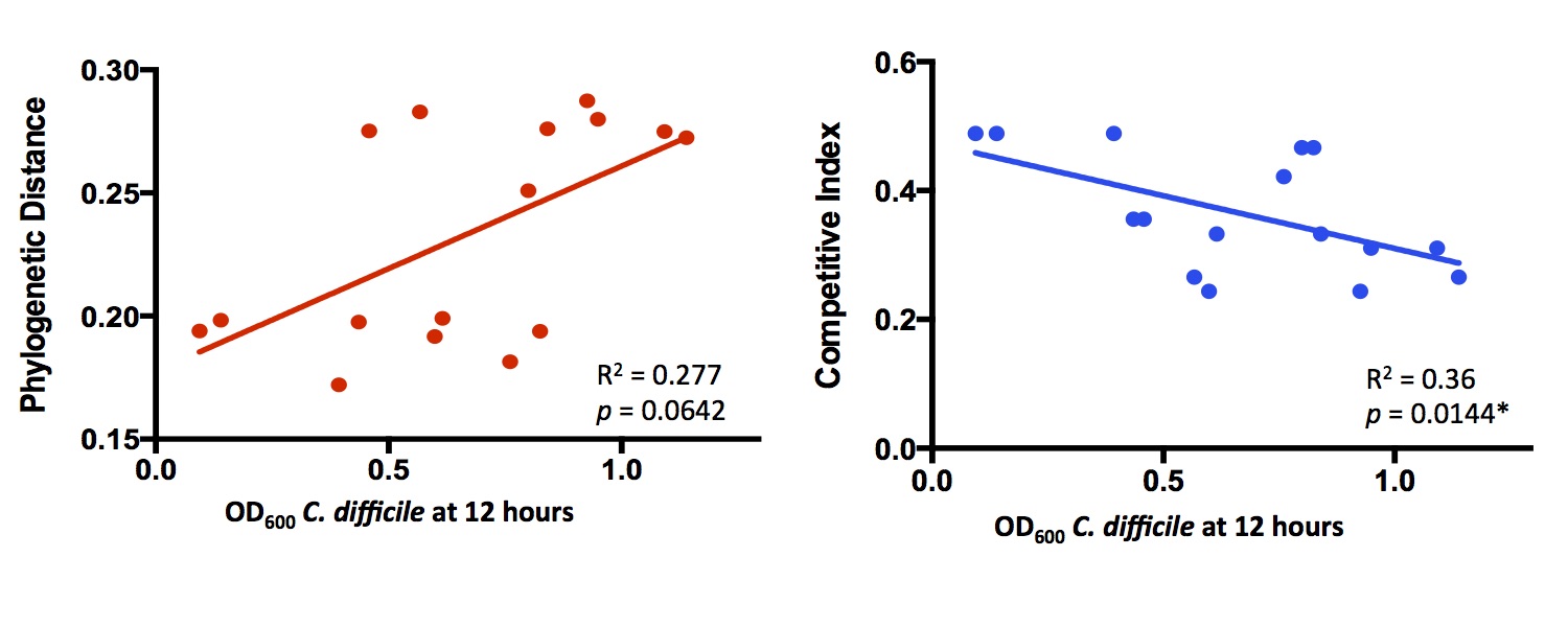
Each point is a separate bacterial species, competed against C. difficile in rich media. Competitive Index refers to how much overlap there is between metabolic networks. I didn’t follow this up much further to focus on other projects, but we may come back to it in the future.
What I’ve been working on more recently has been integrating transcriptomic data into genome-scale metabolic models. The methods I’m using are loosely based on some work I read out of Jen Nielsen’s lab. Their approach used a bipartite network architecture with enzyme nodes connecting to substrate nodes. Since substrates only directly connect to enzyme nodes, you are then able to map transcript abundance to their respective enzymes and then make inferences about how in-demand the substrates they act on are. Here’s part of one network I’ve generated as an example:
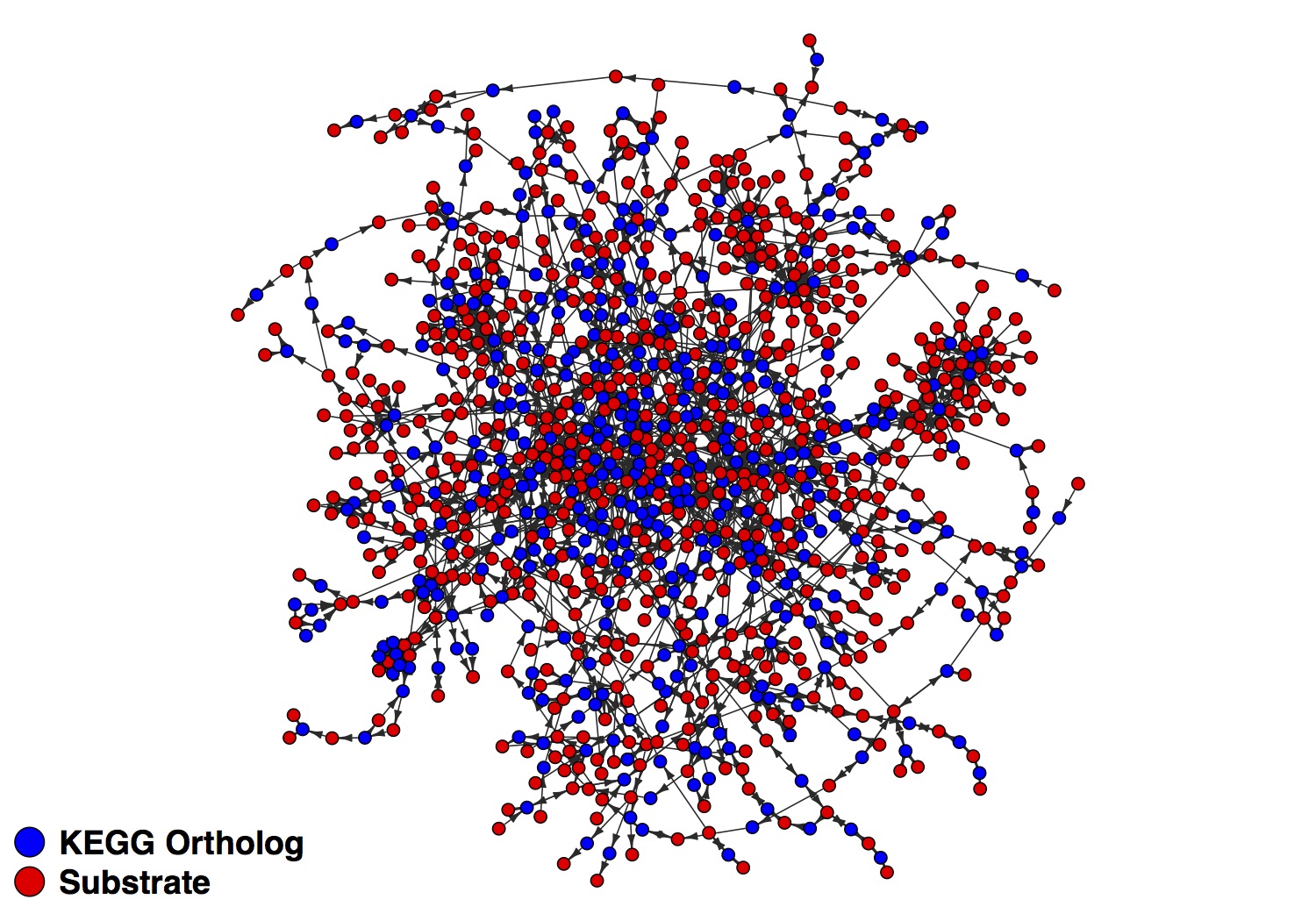
After mapping transcripts to the enzyme (KEGG ortholog) nodes, you can get a read on how important the adjacent substrate nodes are. I’m extending this to infer the nutrient niche of species in the gut. We are working on the analysis and manuscript now so I’ll have a lot more to post soon.
For now, here’s the R code I used to generate the network plot:
# Load igraph package
install.packages("igraph")
library(igraph)

# Define variables
file_name <- '~/bipartite.graph'
nodes_1 <- '~/compound.lst'
nodes_1_label <- 'Substrate'
nodes_2 <- '~/enzyme.lst'
nodes_2_label <- 'KEGG Ortholog'
figure_file <- '~/bipartite.scc.pdf'

# Read in data
graph.file <- read.table(file_name, header = F, sep = '\t')
node_group_1 <- as.vector(read.table(nodes_1, header = F, sep = '\t')$V1)
node_group_2 <- as.vector(read.table(nodes_2, header = F, sep = '\t')$V1)

# Format directed graph
raw.graph <- graph.data.frame(graph.file, directed = T)

# Remove loops and multiple edges to make visualzation easier
simple.graph <- simplify(raw.graph)

# Decompose graph
all.simple.graph <- decompose.graph(simple.graph)

# Get largest component
largest <- which.max(sapply(all.simple.graph, vcount))
largest.simple.graph <- all.simple.graph[[largest]]

# Format data for plotting
V(largest.simple.graph)$size <- 3 # Node size
V(largest.simple.graph)$color <- ifelse(V(largest.simple.graph)$name %in% node_group_2, "blue", "red") # Color nodes
E(largest.simple.graph)$color <- 'gray15' # Color edges

# Plot the network
par(mar=c(0,0,0,0), font=2)
plot(largest.simple.graph, vertex.label = NA, layout = layout.graphopt,
     edge.arrow.size = 0.5, edge.arrow.width = 0.8, vertex.frame.color = 'black')
legend('bottomleft', legend=c(nodes_1_label, nodes_2_label),
       pt.bg=c('red', 'blue'), col='black', pch=21, pt.cex=3, cex=1.5, bty = "n")