There has been a hard stop on posting over the last several months because we were defending our dissertation work, trying to get manuscripts published, starting our postdocs in a new city, and planning a wedding… After a little bit of stress, and even less sleep, my wife and I were able to successfully complete all of these important life milestones together.

Now that we a both onto the next step, I want to take a second to discuss some work that came from my thesis that I’m really proud of. In a nutshell, through a combination of -omics technologies and genome-scale computational modeling, we were able to identify differences in the nutrient niche of C. difficile across separate antibiotic-pretreatment mouse models of infection that correlated with changes in disease severity. What this means is that which antibiotic you are treated with that sensitizes you to C. difficile colonization or what your personel gut community looks like may effect how severely the pathogen impacts you. The article can be found open-access here. This work was also featured as the Editor’s Pick for July 2017 (vol. 2 (4)) and my ternary plot was selected for that issue’s cover! Here was the winning figure:

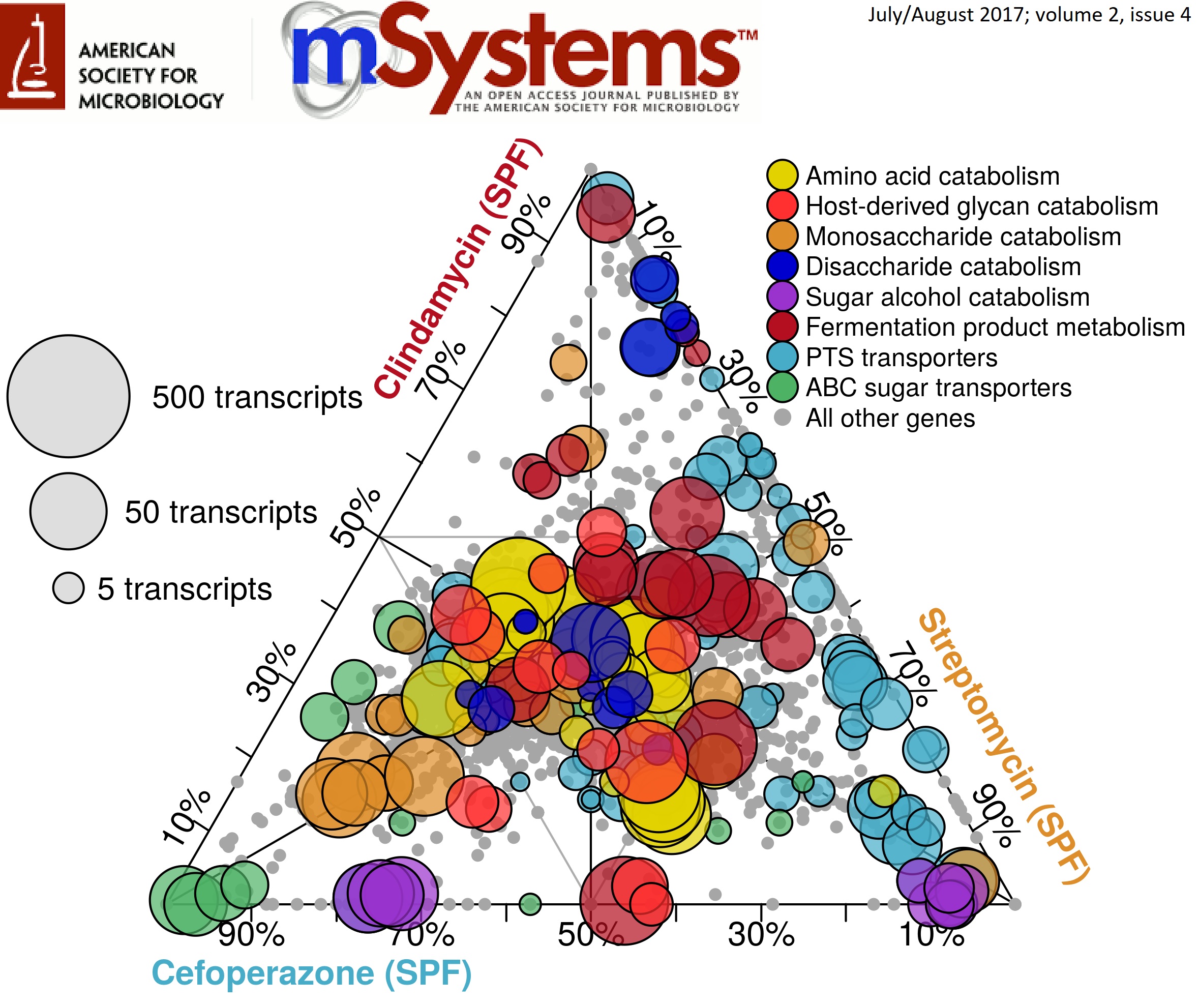
What this figure is showing is the transcript abundance of selected genes in several metabolic pathways across 3 antibiotic pretreatment models. Position of each point reflects the mRNA quantified from each condition associated with each corner. The closer a point is to one edge, the more overrepresented expression of that gene is in that pretreatment group. Size of the points demonstrates the normalized number of transcripts found for that gene in the condition where it’s expression was highest. Overall, this implies that certain forms of metabolism are more active under certain environmental conditions which inform downstream virulence expression. We later confirmed this trend using a simplified metabolic model and untargeted mass spectrometry of metabolites found in the gut during infection.

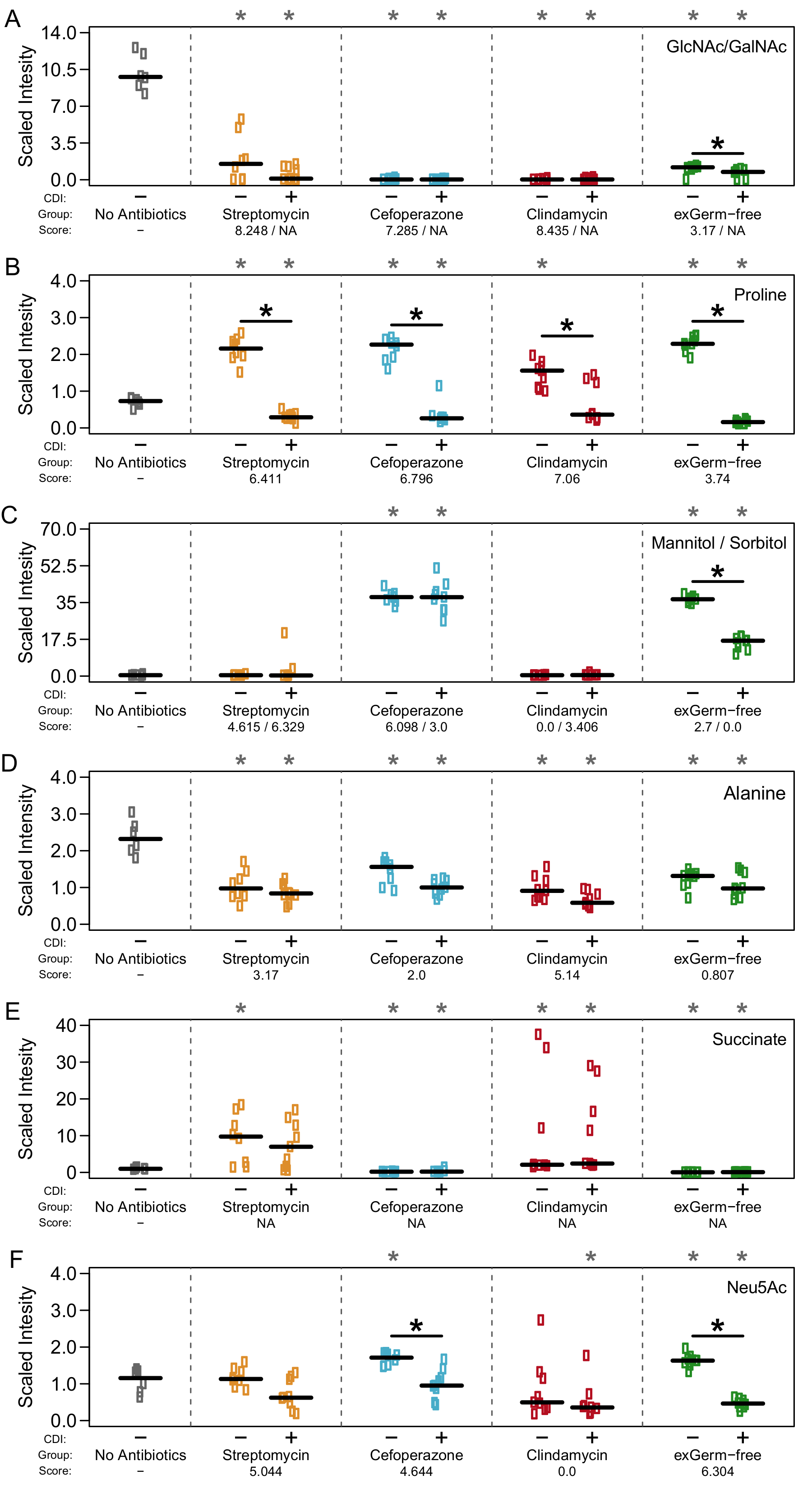
Metabolomic results supported that there was indeed a heirarchy to nutirent preference of C. difficile during infection and this may be determined by which competitors are left over after antibiotics. Check out the rest here!.

It’s time for another post about considerations you should make when tackling a metagenomic or metatranscriptomic dataset. The problem comes in during library construction, even before sequencing. The small amount of PCR cycles that are done to add adapters to the end of the nucleotide fragments is enough to create artifacts during the read mapping process downstream when trying to get a handle on gene or transcript abundance. This is due to the simple fact that when you are look at read mapping counts, you assume that each mapping is an independent event and therefore adds information to your analysis. If PCR duplications are allowed to persist, this is no longer true as multiple reads will map to the same sequence simply because they are exact copies of one another. This can be remedied in a couple of ways…

One method is using an R package called DeSeq within the commonly used Bioconductor. What this program does is basically fit your mapping data to an expected distribution for what an ideal distributioin “should” look like. It looks something like this:

I got this image from a lecture on distributions by Jack Weiss at UNC. This is known as a negative binomial distribution. You can imagine the number of unique genes being on the y-axis, while the number of transcript reads mapping to each on the x-axis. This would illustrate that relatively few genes are being highly transcribed, and most most have low levels of expression. Normalizing to this style of distribution isn’t wrong by any means since all transcript mapping datasets will fit this style of curve if sampled deeply enough, that’s just how biology works. However, it is making some assumptions about your sequencing depth and it doesn’t look at the actual mapping coordinates themselves.

The method I use is a little more robust because it looks at the actually similarity of the mapped reads and decides if they are actually identical or not. You can do this using the MarkDuplicates function within the Picard toolkit. How it works is by scanning through your SAM file and looks for reads with identical 5’ mapping coordinates. Any matches are marked as duplicates and subsequently removed. This relies on the probability that multiple strands of nucleic acid fragmented in the exact same place is so impossibly small that any sequence that starts at the same site is almost definitely due to PCR duplication.

Here is an example of how to run 10 Gb of read data through this kind of PCR dereplication:

1
2
3
4
5
6
7
8
java -Xmx10g -jar /picard/1.77/MarkDuplicates.jar \
INPUT=metatranscriptome.sort.merge.sort.bam \
OUTPUT=metatranscriptome.sort.merge.sort.rmdup.bam \
METRICS_FILE=metatranscriptome.sort.merge.sort.rmdup.metrics \
AS=TRUE \
VALIDATION_STRINGENCY=LENIENT \
MAX_FILE_HANDLES_FOR_READ_ENDS_MAP=1000 \
REMOVE_DUPLICATES=TRUE

After dereplicating a benchmarking dataset, MarkDuplicates found ~75.15% read duplication. This would have heavily skewed my downstream analysis and is a critical step to any transcript mapping study. Here is what the output metrics looked like:

1
2
UNPAIRED_READS_EXAMINED		READ_PAIRS_EXAMINED	UNMAPPED_READS	UNPAIRED_READ_DUPLICATES	READ_PAIR_DUPLICATES	READ_PAIR_OPTICAL_DUPLICATES    PERCENT_DUPLICATION	ESTIMATED_LIBRARY_SIZE
36595704			106878532		61700529	35697350			76225526		61122575			0.751533		53029253

I should note that this data is from a pretty contrived community and other metatranscriptomic datasets are likely <50% duplications, but it’s definitely something to think about when reading these kinds of studies in the future!